Preferential Spatial Gene Expression in Neuroanatomy
Contents
Intro
In this post I will demonstrate how to use my package ABIgeneRMINC to download, read and analyze mouse brain gene expression data from the Allen Brain Institute.
The Allen Brain Institute (ABI) has acquired and released genome-wide spatial gene expression maps for the mouse brain. The data is generated using in situ hybridization experiments (ISH), where nucleotide probes for specific genes bind directly to mouse brain tissue. The probe binding is then marked with a biotin label that can be used to locate regions where a gene is expressed.
For the analysis you will need two R packages RMINC and ABIgeneRMINC.
# devtools::install_github(repo="DJFernandes/ABIgeneRMINC")   # If you need to install
library(ABIgeneRMINC)
library(RMINC)
Getting the data
With the packages load you can now look up your favourite gene. You need to know the gene acronym though, which you can find on the NCBI database. In this case, I want to look up Bdnf. The function below queries the Allen Brain API and finds all experiments conducted with Bdnf.
fge=find.gene.experiment('Bdnf')
fge
## gene slices ExperimentID
## 1 Bdnf sagittal 75695642
## 2 Bdnf coronal 79587720
## URLs
## 1 http://api.brain-map.org/grid_data/download/75695642?include=energy
## 2 http://api.brain-map.org/grid_data/download/79587720?include=energyWe are in luck! There are two experiments the Allen Brain Institute ran with Bdnf, identified by ExperimentIDs 79587720 and 75695642. The former was conducted on coronal slices in the brain, and the latter on sagittal slices. We will see why this is important later on. The URLs where you can download expression data is given in the final column. You can enter them in your internet browser and file should begin to download. If you don’t want to leave the wonderful world of R just to download (I don’t blame you), we can actually download and read the data within R itself.
genedata1 = read.raw.gene(as.character(fge$URLs[1]),url = TRUE)## Loading required package: bitopsIt is generally better to download outside R and save the file, so you don’t have to keep downloading. Obtain the path to the file, and use it as as argument to read as follows:
genedata1 = read.raw.gene('/projects/egerek/matthijs/2015-07-Allen-Brain/Allen_Gene_Expression/raw_data/coronal/Bdnf_sid79587720/energy.raw')Visualizing the gene expression
The gene expression data is a 1D vector. It can easily be converted to a 3D array using the mincArray function (which we will do later). But there is an important note to talk about before going further. The 1D vector lists values going from X=Anterior-to-Posterior, Y=Superior-to-Inferior, and Z=Left-to-Right (dimensions written from fastest changing index to slowest). This is the ABI orientation. The RMINC vectors typically are 1D vectors going from X=Left-to-Right, Y=Posterior-to-Anterior, Z=Inferior-to-Superior (dimensions written from fastest changing index to slowest). This is the MNI orientation. You can make a choice as to which orientiation you want to analyze in but I will be choosing MNI orientation in this tutorial. Just make sure you are consistent with your orientations and you won’t have problems. The function below converts ABI orientation to MNI orientation:
genedata1 = allenVectorTOmincVector(genedata1)
# genedata1 = mincVectorTOallenVector(genedata1)  #This is the inverse function
Now, we can visualize the gene expression. Below is a sagittal slice
image(mincArray(genedata1)[30,,], ylab='Superior-Inferior' ,xlab='Anterior-Posterior')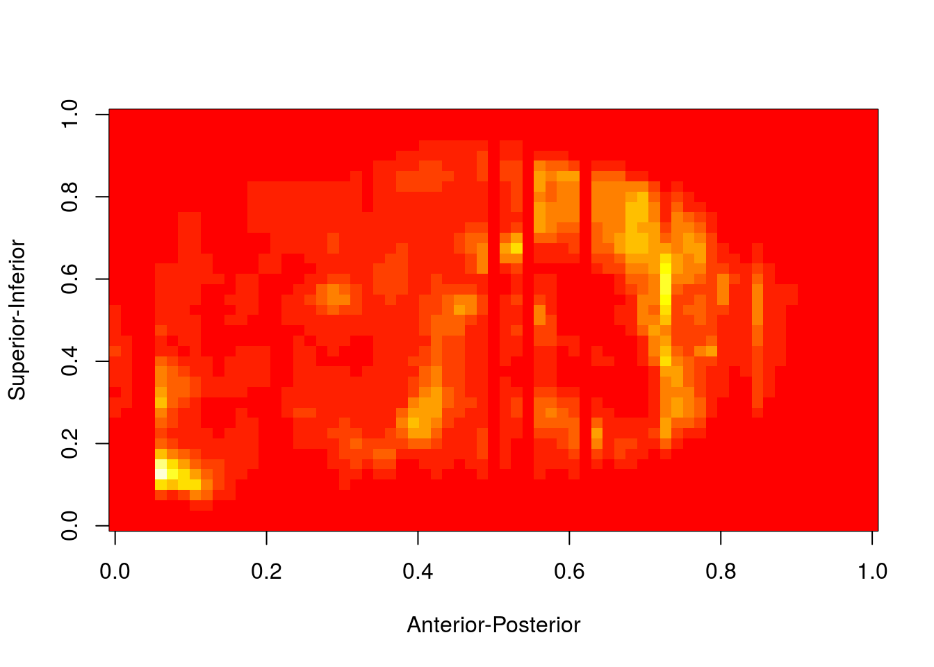
Adding an anatomical underlay
I am not a good mouse brain anatomist, and so I find it pretty difficult to tell from this expression heatmap where exactly the expression is in the brain. We will now overlay a background MRI template to tell us where the gene expression is and use RMINC to create slice series.
anatfile='/projects/egerek/matthijs/2015-07-Allen-Brain/allenCCFV3_to_dorr_registration/allenCCFV3/atlas_in_200um/Dorr_resampled_200um.mnc'
mincPlotSliceSeries(
  anatomy=mincArray(mincGetVolume(anatfile)),
  statistics=mincArray(genedata1),
  symmetric=FALSE,
  col=colorRampPalette(c("darkgreen","yellowgreen"))(255),
  legend="Bdnf Expression",low=2,high=6.5)
Much better. I can tell there is high expression in the cortex and hippocampus.
Let us also look at the other Bdnf experiment (ID: 75695642).
genedata2 = read.raw.gene(as.character(fge$URLs[2]),url = TRUE)
genedata2 = allenVectorTOmincVector(genedata2)
mincPlotSliceSeries(
  anatomy=mincArray(mincGetVolume(anatfile)),
  statistics=mincArray(genedata2),
  symmetric=FALSE,
  col=colorRampPalette(c("darkgreen","yellowgreen"))(255),
  legend="Bdnf Expression",low=2,high=6.5)
We see that the sagittal slices only span half the brain. This was a deliberate choice by the ABI and most of the gene experiments are like this. Furthermore, slices are sampled every 200 microns for the sagittal datasets and every 100 microns for the coronal datasets. That is why we prefer using the coronal slices any chance we get, but there are still tools that help us work with sagittal data. We can reflect data across the sagittal midplane to fill in the missing hemisphere as so:
genedata2.reflected=midplane.reflect(genedata2,reflect.dim=3)
mincPlotSliceSeries(
  anatomy=mincArray(mincGetVolume(anatfile)),
  statistics=mincArray(genedata2.reflected),
  symmetric=FALSE,
  col=colorRampPalette(c("darkgreen","yellowgreen"))(255),
  legend="Bdnf Expression",low=2,high=6.5)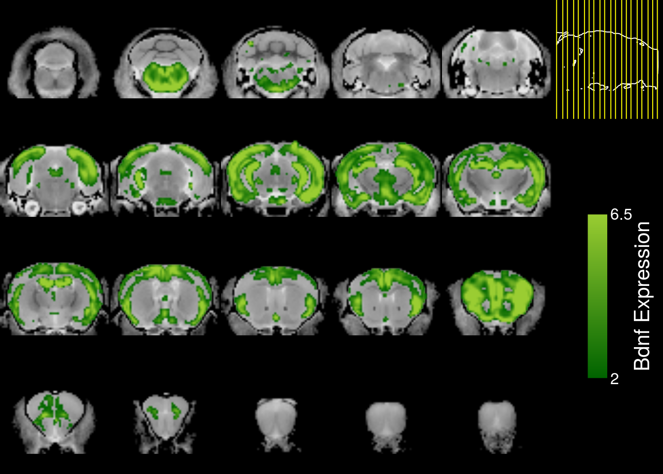
We can do better. Because there sagittal sections were only sampled every 200um, there is a lot of missing data due to slice misalignment. We can fill them in using nearest neighbour marching averages.
labelfile=system.file('extdata/gridAnnotation.raw',package="ABIgeneRMINC")
mask=allenVectorTOmincVector(read.raw.gene(labelfile,labels=TRUE)>0)
interp.gene=interpolate.gene(genedata2.reflected,mask)

mincPlotSliceSeries(
  anatomy=mincArray(mincGetVolume(anatfile)),
  statistics=mincArray(interp.gene),
  symmetric=FALSE,
  col=colorRampPalette(c("darkgreen","yellowgreen"))(255),
  legend="Bdnf Expression",low=2,high=6.5)
Even with interpolation, the expression map is not that good.
Expression statistics
Moving back to the coronal maps, let’s generate summary statistics for each structure in the ABI atlas.
labels=read.raw.gene(labelfile,labels=TRUE)
labels.to.sum=sort(unique(labels))
labels.to.sum=labels.to.sum[labels.to.sum!=0]

udf=unionize(grid.data=genedata1,             #vector to unionize
           labels.to.sum=labels.to.sum,       #sum all labels
           labels.grid=labels                 #the vector of labels
           )
udf=udf[order(udf$mean,decreasing=TRUE),]
head(udf)
## labels sum mean stdev
## 167 287 19.641589 4.910397 12.018447
## 474 875 48.372759 4.397524 6.287998
## 261 483 123.968708 3.178685 3.827543
## 171 292 34.930620 3.175511 6.002760
## 162 279 6.248917 3.124459 3.977935
## 22 50 12.193722 3.048430 1.094984Now let us read a csv with structure names in it that correspond to the label number and add that as a column in our data frame.
labeldefs=read.csv("/projects/egerek/matthijs/2015-07-Allen-Brain/Allen_Gene_Expression/labels/allen_gridlabels_structures.csv") #this can be downloaded from ABI
udf$structures=labeldefs[match(labeldefs$id,udf$labels),'name']
udf = udf[,c('structures','labels','mean','sum','stdev')]
head(udf)
## structures
## 167 Main olfactory bulb, outer plexiform layer
## 474 Bed nuclei of the stria terminalis, anterior division, anterolateral area
## 261 Visceral area, layer 6b
## 171 Uvula (IX), granular layer
## 162 Retrosplenial area, lateral agranular part, layer 1
## 22 Bed nuclei of the stria terminalis, anterior division, oval nucleus
## labels mean sum stdev
## 167 287 4.910397 19.641589 12.018447
## 474 875 4.397524 48.372759 6.287998
## 261 483 3.178685 123.968708 3.827543
## 171 292 3.175511 34.930620 6.002760
## 162 279 3.124459 6.248917 3.977935
## 22 50 3.048430 12.193722 1.094984Voila, we can now tell which structures have high gene expression for the gene we are interested in.
Outro
I plan to do tutorials on more fancy gene expression analyses in the future, but this is the base from which future tutorials will be built. I hope this gets you started on using gene expression to explore neuroanatomical phenotypes and gives you an understanding of some of the caveats associated with spatial gene expression analysis.