Why Relative Volumes Matter
Contents
Intro
Figuring out how one group’s brain is different from another’s is a big part of neuroscience. MRI-neuroanatomy – the study of the sizes of brain regions – is a wonderful tool for this job and makes up a sizeable chunk of what we study. MRI operates in a lovely middle ground in the scales of neuroscience. It is strongly related to macroscale features of the organism, including sex, behaviour, etc; but can also inform us about the effects of microscale factors – such as gene expression.
While neuroanatomy is tremendously advantageous in the study of what makes one group’s brain is different from another’s, it is ill-suited to the question of why they are different. It is ultimately the question of mechanism – the why – that drives science forward. However, the fact that neuroanatomy can’t identify mechanism doesn’t make it useless. This blog will detail one way that neuroscience benefits from the neuroanatomy.
The pursuit of why begins with the question of what.
Brain Volumes
There are two types of sizes when one typically talks about brain volumes. The first is absolute size (or absolute volume) which is typically measured in cubic millimeters. This is the true volume of a brain region. The second is relative size (or relative volume), which is the absolute volume divided by whole-brain volume. Both measures have their advantages and disadvantages, however the advantage of relative volume may not be readily apparent. Absolute volumes are built from local microscale properties such as neurons, glia, the dendritic tree, etc. It is the sum of these microscale properties that determines the absolute volume of a region and ultimately contributes to the size of the brain. Relative volumes, on the other hand, normalise to whole brain size and, therefore, don’t have any trivial local influences. This issue of locality naturally leads to a criticism that relative volumes are meaningless compared to absolutes as they can’t help us infer localized changes. This cirticism may appear true at face value, but a closer inspection of real data reveals subtle nuances that strengthen the case for relative volumes.
The Data
The data we will be examining – graciously provided by Lily Qiu – is neuroanatomy data comparing male and female mice over a comprehensive period of neurodevelopment spanning nine timepoints ranging from p3 (i.e 3-day-old mouse, which corresponds to a human fetus) to p65 (i.e 65-day-old mice, which corresponding a human adult). In order to evaluate whether absolute volumes or relative volumes are more useful to study sex differences in the brain, we employed techniques from machine learning to develop a classifier that predicts sex from neuroanatomical structure volumes at a particular age. First, we excluded one mouse’s neuroanatomy data and fit a LASSO logistic regression to simulataneously perform feature selection and predict sex from neuroanatomy. Once trained, the model was then provided the excluded mouse’s data to test whether it could successfully predict the excluded mouse’s sex. We repeated this process for every mouse and every age, training a unique classifier each time. Importantly, each classifier was always assessed for accuracy on data it had not seen during training. We trained one set of classifiers to predict sex from absolute volumes and another set to predict sex from relative volumes. Figure 1 shows the accuracy of the classifier and we see that for most ages, classifiers trained using relative volumes predicted sex better than those trained with absolute volumes. More importantly, relative-based classifiers vastly out-performed their absolute-based counterparts at the early ages between 3-17 (p17 corresponds to a human child). While absolute volumes may have a favorable interpretation, an unbiased machine learning procedure favors studying sex differences in terms of relative volumes. Absolute volumes may actually be biased against sex differences at the early ages between p3-17.
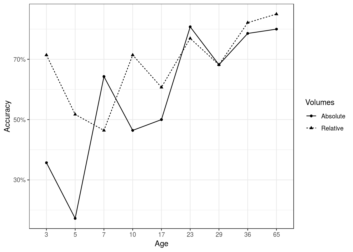
Figure 1: Relative volumes predict sex better than absolute volumes, especially p3-p17.
To understand why the classifier performs better with relative volumes over absolute volumes, it is instructive to look at Figure 2, which plots the Coefficient of Variation (CV) over time for the Bed Nucleus of the Stria Terminalis (BNST) measured using absolute and relative volumes. CV is the standard deviation divided by the mean and is therefore unitless. In the BNST, as well as other brain regions, we see a clear pattern where the young brain has high CV in their absolute volumes but remarkably stable CV in relative volumes, therefore explaining why classifiers based on relative volumes outperformed their absolute counterparts at young ages. This consistent low CV is what makes relative volumes so useful in studying sexual dimorphisms. The young brain has quite a lot of variability in growth between subjects that relative volumes effectively correct for. Once corrected, the subtle neuroanatomy that distinguishes males and females becomes clearer to the LASSO-based classifiers. The correction also makes statistical modelling easier as well, as illustrated by Figure 3. The greater variability in the young brain masks statistics relating to when absolute volume sexual dimorphisms emerge, thereby providing a delayed estimate as to when male BNST becomes larger than females (around p10-p17). Relative volumes, however, have sexual dimorphisms emerge much earlier (p5), which is close to and supported by extensive histological evidence. Finally, relative volumes also scale away the overall growth of the brain and can therefore be approximated using linear models. Abolute volumes, on the other hand, need to be fitted with non-linear function, especially when considering their growth throughout a comprehensive period of neurodevelopment. While, in this case, non-linear fitting is not really an issue for statistical significance, the additional degrees-of-freedom needed to properly fit non-linear curves might be too costly in studies with less subjects.
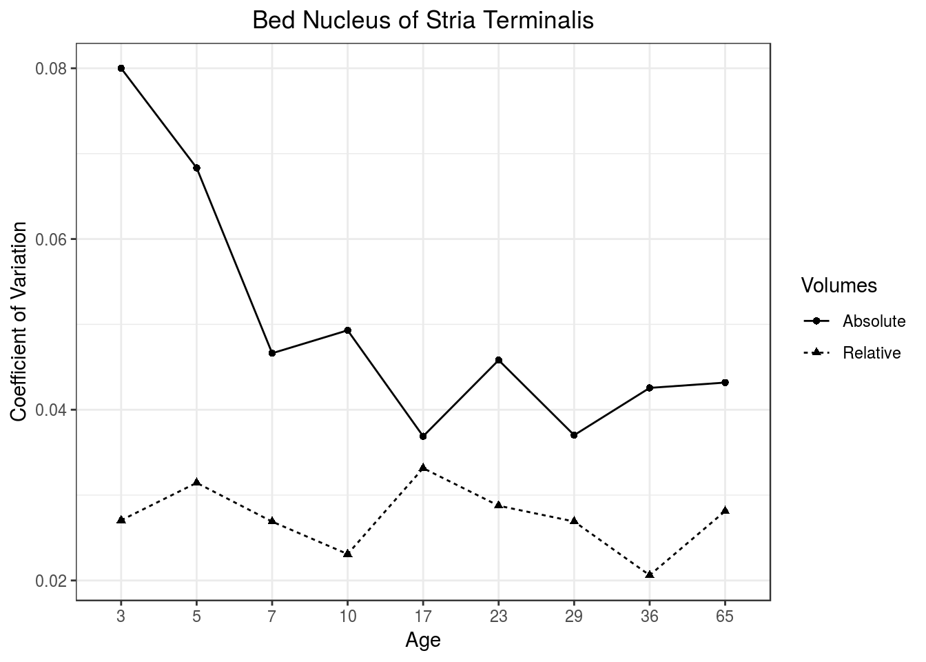
Figure 2: Relative volumes have low coefficient of variation over the neurodevelopment time period.
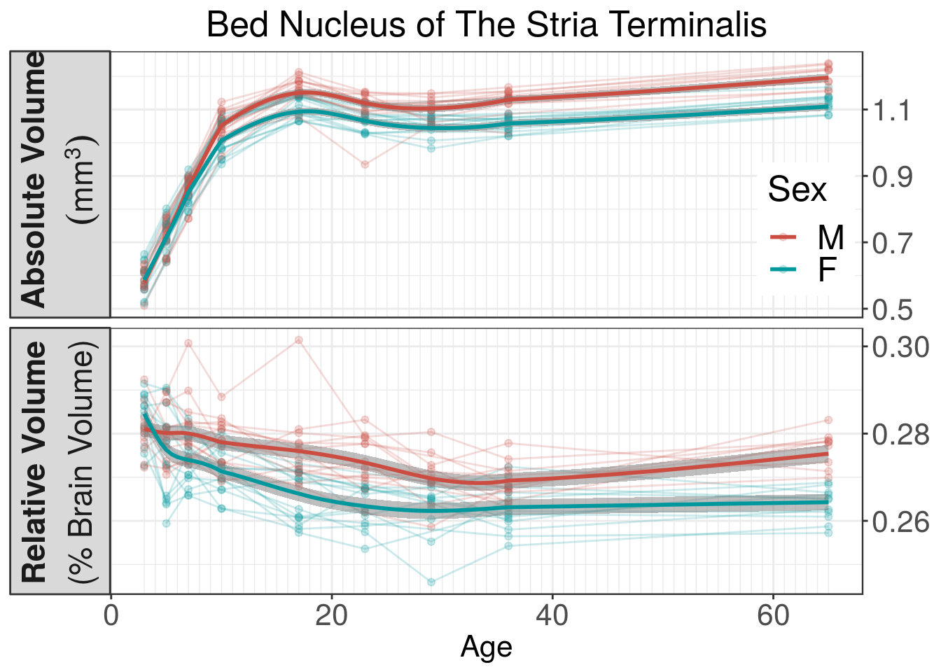
Figure 3: Volume of the BNST over time. We see with absolue volumes that sexual dimorphisms emerge between p10 and p17. Relative volumes on the other hand have dimorphisms emerging around p5. Extensive histological evidence in literature supports the timing of relative volume sexual dimorphisms. Shaded regions represent standard error estimated from linear mixed-effect models.
What about the issue of locality I mentioned earlier? Absolute volumes are guaranteed to have local causes, but relative volumes do not. While it is certainly true that relative volumes may have nonlocal causes, we find that nonlocal effects are either exceedingly small in a mouse or rare in a proper image registration procedure. To illustrate relative volumes, please consider Figures 4 and 5. We showed the relative and absolute determinants for a registration of the p3 average mouse brain and the p5 average mouse brain. In both relative and absolute determinants, there is a great deal of agreement as to which structures have a high degree of change from p5 to p3 (cerebellum, cortex, olfactory bulb). Therefore, local causes that affect absolute determinants would affect relative volumes as well. In summary, both relative and absolute volumes are important for volume analysis depending on the situation. Relative volumes are useful when there is a high degree of variation in brain sizes obscuring potentially interesting effects and are generally easier to model. Absolute volumes on the other hand provide information in cannonical units that may be more intuitive to other researchers. Even with just these two measures, we can already get a glimpse into what is happening in the young mouse brain. There is a high degree of variability in the young mouse brain that becomes less noticable with time. Why does this variability exist? The answer is unclear but it could be related to the uterine position and horn size (McLaurin, et al. 2015). What can this young variability tell us about the adult mouse? This question can be explored with neuroanatomy.

Figure 4: Registration of a source image (p03 average) to a target (p05 average). The native images (after rigid alignment) are on the top row and their overlay is in the middle column. Poor alignment can be found in structures like the cerebellum where there is rapid neonatal growth. Affine registration scales and shears the source image to better align with target image. The affine transformation (generated from the affine registration) is applied to the source image and is shown in the second row. The overlay shows a good match between the affine-transformed source and the target images. However, zooming into the cerebellum of the affine-transformed source and target image (third row), shows that affine registration does not produce proper alignment of the cerebellum. This is illustrated by applying a red contour to the cerebellum of the target image and overlaying this contour to the source image. The non-affine registration corrects this discrepancy (fourth row) and produces the best alignment between source and target images (fifth row).

Figure 5: Visualizing deformations caused by transformation of target image using grids and determinants. Illustrated in the left figure, upon transformation of the target image to the source image (this transformation is the inverse of the transformation in Figure 4), gridlines in the target image become warped. In the top row, the gridlines warp from transformation to the source image; and in the bottom row, the gridlines warp from transformation to the affine-transformed source. Volumetric changes caused by the transformation can be qualitatively assessed by observing how the volume of a square region (region defined by the open space between gridlines) changes after transformation. Absolute determinants capture volumetric changes upon transformation between the Target and Native Source images. Relative determinants capture volumetric changes upon transformation between the Target image and Source image after affine transformation.
A major criticism of neuroanatomy analysis is that mouse models are useful for the study of cellular mechanisms; and strictly studying brain volumes does not take advantage of what makes mouse research so useful. This criticism ignores the myriad number of informative analysis that mouse models make possible and I will be describing one such analysis in the remainder of this blog. In vivo longitudinal imaging throughout mouse neurodevelopment (provided by Lily Qiu’s data), in conjunction with the control of genetic and environmental factors afforded by mouse studies, renders it possible to explore exciting analysis in brain prediction. Neuroanatomy of the young mouse brain predicts neuroanatomy of the adolescent and adult mouse brain (I will show our work in more detail in a future blogpost). By developing a computational model to predict mouse brain neuroanatomy, we found that only the first 10-17 days of neuroanatomical data are enough to make sensitive and specific predictions of individualised neuroanatomy at p36 and p65. As expected, if we provide the model with only p03 data and ask it to predict p36 or p65, the model will fail to make specific predictions because young brains’ variability is not very informative. However, the more data we provide from later in development, the better the model is at identifying features of variability unique to a mouse and predicting mature individualised neuroanatomy. It is through a combination of many timepoints and more recent timepoints that individual differences in young neuroanatomy emerge, which the model can use to make predictions about mature neuroanatomy. Our prediction accuracies were not influenced by the sex of the predicted subject (i.e. males and females are equally well predicted), however, we found that male neuroanatomy individualised (became easier to predict) significantly earlier in development than female neuroanatomy.
Neuroanatomical phenotyping tends to be used to study how groups of organisms are similar. However, it is also important to study what makes organisms unique from the rest of the members of its group. The control of genetic and environmental factors limits the variability in mice making it easier for machine-learning tools to make individualised predictions. “Easier” in this context means using simple models and few subjects. While humans have far more variability compared to mice, with the advent of ever-bigger datasets collected on human neurodevelopment, it will be possible in the near future to use more advanced machine-learning tools to predict some individuality in these data sets. It might even be possible to predict the development of neuroanatomical pathologies associated with neurological disorders prior to disorder onset. Neuroanatomy research in mouse models can spur research in this exciting direction. Neuroanatomy can be a marker for individaulity: what makes mice different from other mice and humans different from other human. I can hardly wait for future science to determine why.