Linear Models: Understanding the Error Estimates for Binary Variables
Contents
Introduction
library(tidyverse)
library(matlib)
library(knitr)
library(RColorBrewer)
The purpose of this document is to understand the parameter and residuals error estimates in a basic linear regression model when working with binary categorical variables. Recall the general model definition:
\[ \mathbf{y} = \mathbf{X}\mathbf{\beta} + \mathbf{e}\]
where \(\mathbf{X}\) is the design matrix and \(\mathbf{\beta}\) is a \((p+1)\)-vector of coefficients/parameters, including the intercept parameter. The errors are normally distributed around 0 with variance \(\sigma^2\):
\[e \sim N(0,\sigma^2) \quad .\]
Upon fitting the model to data, we obtain estimates for the coefficients, \(\hat{\beta}\). These estimates have an associated covariance matrix \(\sigma^2_\beta\), which is used for statistical inference. The covariance matrix of the parameters is calculated from the estimate for the residual standard error in the following way:
\[\mathbf{\sigma}^2_\beta = (\mathbf{X}'\mathbf{X})^{-1}\hat{\sigma}^2 \quad .\]
The focus of this document will be on understanding the details of this covariance matrix, specifically of the parameter standard errors and the residual standard error, \(\hat{\sigma}\). The squared parameter standard errors (i.e. parameter variances) are the diagonal terms in the covariance matrix, and so the two measures of variability are related to one another in the following way:
\[\text{diag}[\mathbf{\sigma}^2_\beta] = \text{diag}[(\mathbf{X}'\mathbf{X})^{-1}]\hat{\sigma}^2 \quad .\]
The standard errors can then be obtained by taking the square root of the variances. This transformation between the residual standard error and the parameter standard errors is not trivial and depends on the number of parameters and type of variables. Recall that the estimate for \(\sigma\) is given by
\[\hat{\sigma}^2 = \frac{1}{n-p-1} \sum_{i = 1}^n e^2_i \quad .\]
If the data includes observations of categorical variables such that it can be pooled into balanced groups with potentially different group sample standard deviations of \(\sigma_g\), it can be shown straightforwardly that if \(n \gg p\), i.e. in the regime of low-dimensional data,
\[\hat{\sigma}^2 = \text{Ave}[\sigma^2_g] \quad .\]
If the sample standard deviations of the groups are identical, then \(\hat{\sigma} = \sigma_g\). What this tells us is that the residual standard error is an estimate on the standard deviation of the groups defined by the model.
We will get a sense of how these estimates vary by generating some simulated data and playing with different linear models of the data. In particular, we will simulate a balanced experimental design consisting of independent binary categorical variables and a continuous response. We will consider three binary variables: Genotype, Anxiety, and Treatment. The use of binary variables in linear models has the effect of pooling the data across different groups. Since there are 3 binary variables, there will be 8 separate groups, i.e. \(2^3\). To operate well within the low-dimensitonality regime, we will use a large sample size. The data will be simulated by first generating a scaffold data frame containing the observations for the different categorical variables. The scaffold data frame will then be used to generate the response variable stochastically. We will start by generating the scaffold data frame.
#Define variables related to the experimental design.
# Sample size
nSample <- 100
# Number of binary variables
nBinVar <- 3
# Number of distinct groups
nGroups <- 2^nBinVar
#Total number of observations
nObs <- nSample*nGroups

#Generate data frame (handy trick uisng expand.grid() and map_df())
dfGrid <- expand.grid(Genotype = c("WT","MUT"),
                      Anxiety = c("No","Yes"),
                      Treatment = c("Placebo", "Drug"))
dfSimple <- map_df(seq_len(nSample), ~dfGrid) %>%
  mutate(Genotype = factor(Genotype, levels = c("WT","MUT")),
         Anxiety = factor(Anxiety, levels = c("No","Yes")),
         Treatment = factor(Treatment, levels = c("Placebo","Drug")))

#Verify that this worked
dfSimple %>%
  group_by(Genotype, Anxiety, Treatment) %>%
  count
## # A tibble: 8 x 4
## # Groups: Genotype, Anxiety, Treatment [8]
## Genotype Anxiety Treatment n
## <fct> <fct> <fct> <int>
## 1 WT No Placebo 100
## 2 WT No Drug 100
## 3 WT Yes Placebo 100
## 4 WT Yes Drug 100
## 5 MUT No Placebo 100
## 6 MUT No Drug 100
## 7 MUT Yes Placebo 100
## 8 MUT Yes Drug 100Now we create the distribution of the response based on the independent variables. We will generate data in which there are no interactions between any of the predictor variables. The response will be generated using standardized units so that it can stand in for any physical variable. The main effects of the predictors on the response are taken to be \(2\sigma\), where \(\sigma\) is the standard deviation of the normal distribution used to generate observations of the response.
#Simulation parameters
meanRef <- 0
sigma <- 1
effectGenotype <- 2*sigma
effectAnxiety <- 2*sigma
effectTreatment <- 2*sigma

#Generate data based on experimental design.
#In this case, no interaction between variables.
dfSimple$Response <- meanRef +
  effectGenotype*(as.numeric(dfSimple$Genotype)-1) +
  effectAnxiety*(as.numeric(dfSimple$Anxiety)-1) +
  effectTreatment*(as.numeric(dfSimple$Treatment)-1) +
  rnorm(nrow(dfSimple), 0, sigma)

ggplot(dfSimple, aes(x = Genotype, y = Response, col = Anxiety)) +
  geom_jitter(width = 0.2) +
  facet_grid(.~Treatment) +
  scale_color_brewer(palette = "Set1")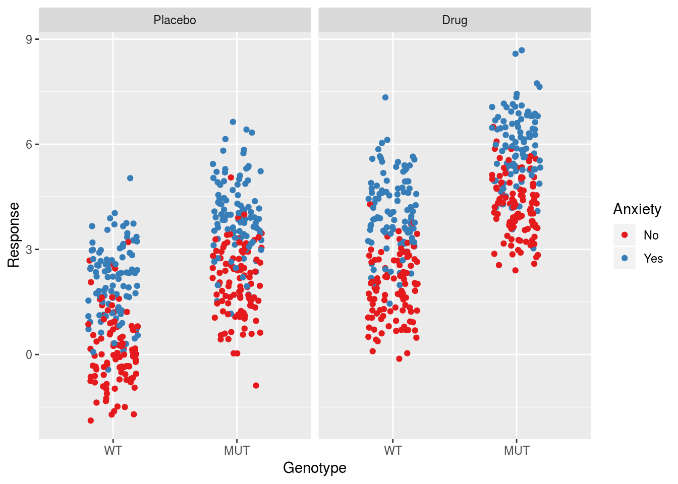
With the data generated we can start considering different linear models to understand the error/variance estimates. In the following Sections we will consider models with and without interactions to examine how the error estimates change. The general process will be to run a given model on the simulated data and examine the details of the transformation from \(\sigma\) to \(\sigma_\beta\) for that model. In doing so we will see that a number of patterns emerge.
Non-interactive Models
Model 1: Intercept Term Only
The first model is one where the only parameter is the intercept. The \(\beta\) estimate returned will be the mean of the data pooled across all groups. The distribution of the pooled response observations is as follows:
ggplot(dfSimple, aes(x = Response)) +
  geom_histogram(binwidth = 1,
                 alpha = 0.7,
                 col = "black",
                 fill = brewer.pal(3,"Set1")[2])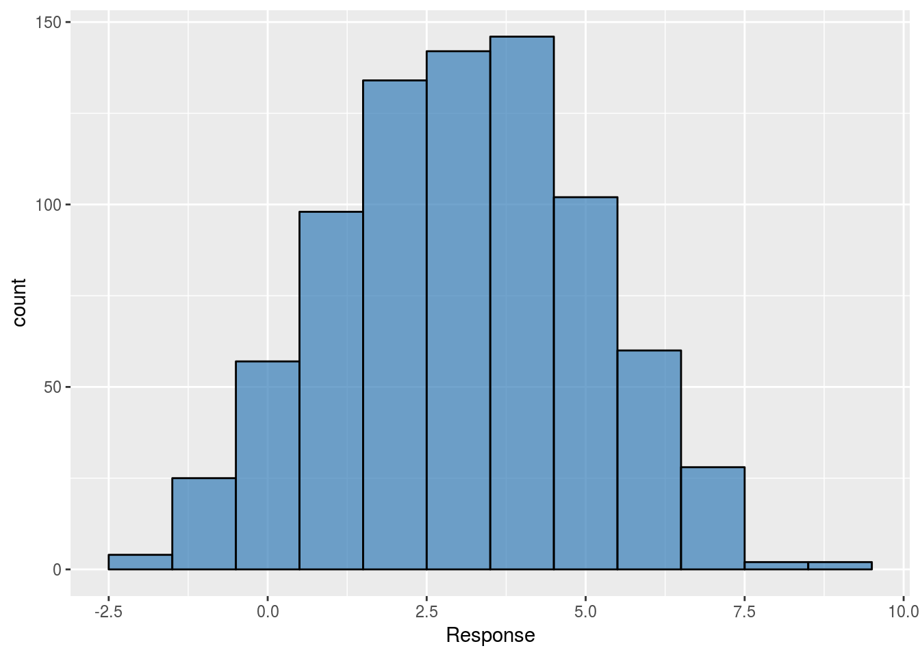
The model is written as
linMod1 <- lm(Response ~ 1, data = dfSimple)
summary(linMod1)
##
## Call:
## lm(formula = Response ~ 1, data = dfSimple)
##
## Residuals:
## Min 1Q Median 3Q Max
## -4.9321 -1.4254 0.0717 1.3874 5.6359
##
## Coefficients:
## Estimate Std. Error t value Pr(>|t|)
## (Intercept) 3.04683 0.07026 43.36 <2e-16 ***
## ---
## Signif. codes: 0 '***' 0.001 '**' 0.01 '*' 0.05 '.' 0.1 ' ' 1
##
## Residual standard error: 1.987 on 799 degrees of freedomIn this simple case, the residual standard error is simply the standard deviation of the full data:
dfSimple %>%
  summarise(sd(Response))
## sd(Response)
## 1 1.987383What about the standard error of the intercept?
Since there is only one parameter for the intercept, the design matrix will just be a vector of ones. The transformation \(\mathbf{X}'\mathbf{X}\) is then just the squared norm of the vector and will be equal to the number of observations in the data set, i.e. \(\sum_{i=1}^n 1 = n\). The inverse operation is just that for a scalar value and we get \(\sigma_\beta = \frac{\sigma}{\sqrt{n}}\). Multiplying the standard error estimate by \(\sqrt{n}\) should return the value of the residual standard error:
summary(linMod1)$coefficients[["(Intercept)","Std. Error"]]*sqrt(nObs)## [1] 1.987383Model 2: One Binary Predictor
Next we add one of the binary variables as a predictor in the model. This will have the effect of pooling the data according to the different levels of that predictor.
ggplot(dfSimple, aes(x = Genotype, y = Response)) +
  geom_jitter(width = 0.2,
              col = brewer.pal(3,"Set1")[2])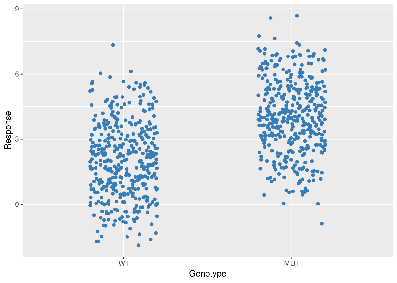
In this case the intercept estimate will indicate the pooled mean of the wildtype group (or whatever the reference level is for the chosen predictor) and the slope estimate will indicate the difference between the wildtype mean and the pooled mean of the mutant group.
linMod2 <- lm(Response ~ Genotype, data = dfSimple)
summary(linMod2)
##
## Call:
## lm(formula = Response ~ Genotype, data = dfSimple)
##
## Residuals:
## Min 1Q Median 3Q Max
## -4.933 -1.212 -0.024 1.215 5.291
##
## Coefficients:
## Estimate Std. Error t value Pr(>|t|)
## (Intercept) 2.04567 0.08588 23.82 <2e-16 ***
## GenotypeMUT 2.00231 0.12145 16.49 <2e-16 ***
## ---
## Signif. codes: 0 '***' 0.001 '**' 0.01 '*' 0.05 '.' 0.1 ' ' 1
##
## Residual standard error: 1.718 on 798 degrees of freedom
## Multiple R-squared: 0.2541, Adjusted R-squared: 0.2532
## F-statistic: 271.8 on 1 and 798 DF, p-value: < 2.2e-16What do the variance estimates represent? Remember that the residual standard error is an estimate of the variability across all of the data. As mentioned in the introduction, the residual standard error will be the square root of the average of the sample variances of the two groups. The group variances and the resulting standard error estimate are:
dfSimple %>%
  group_by(Genotype) %>%
  summarise(varPerGroup = var(Response)) %>%
  ungroup() %>%
  mutate(sigma = sqrt(mean(varPerGroup)))
## # A tibble: 2 x 3
## Genotype varPerGroup sigma
## <fct> <dbl> <dbl>
## 1 WT 3.01 1.72
## 2 MUT 2.89 1.72Which is equal to the estimate for the residuals standard error.
How do the standard errors of the parameters relate to the residual standard error for this model? Let’s compute the transformation explicitly using the design matrix. First we compute \(\mathbf{X'X}\):
xMat <- model.matrix(linMod2)
t(xMat)%*%xMat
## (Intercept) GenotypeMUT
## (Intercept) 800 400
## GenotypeMUT 400 400Indicating the number of observations explicitly, we can see that this matrix is of the form:
\[\mathbf{X}'\mathbf{X} = n \cdot \begin{bmatrix} 1 & \frac{1}{2} \\ \frac{1}{2} & \frac{1}{2} \end{bmatrix}\]
Taking the inverse (which is a straightforward process for a 2x2 matrix such as this) and multiplying by \(\sigma\), we find that the covariance matrix is
\[\sigma^2_\beta = \frac{\sigma^2}{n} \cdot \begin{bmatrix} 2 & -2 \\ -2 & 4 \end{bmatrix}\]
Specifically, the standard errors of the estimates are given by the square roots of the diagonal terms in this matrix (note that this isn’t a proper matrix operation but think of this as extracting the diagonal elements and then taking the square root of each of them):
\[\sigma_\beta = \frac{\sigma}{\sqrt{n}}\begin{bmatrix} \sqrt{2} & \sqrt{4} \end{bmatrix}\]
A point of interest here is that the parameter errors are related to this quantity \(\frac{\sigma}{\sqrt{n}}\) but are scaled by some multiplicative factor. Notably, the slope parameter is more uncertain than the intercept. Multiplying the parameter standard errors by the appropriate multiplicative factors, we should recover the residual standard error:
vec <- c(sqrt(nObs/2), sqrt(nObs/4))
summary(linMod2)$coefficients[,"Std. Error"]*vec
## (Intercept) GenotypeMUT
## 1.717502 1.717502Model 3: Two Binary Predictors
In our third model, we consider the effects of two binary predictors without an interaction. This will pool the data into the \(2^2=4\) groups defined by these predictors:
ggplot(dfSimple, aes(x = Genotype, y = Response, col = Anxiety)) +
  geom_jitter(width = 0.2) +
  scale_color_brewer(palette = "Set1")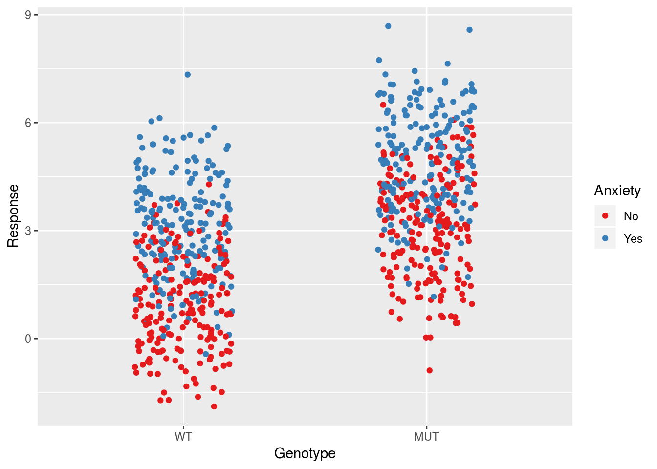
The model is as followed:
linMod3 <- lm(Response ~ Genotype + Anxiety, data = dfSimple)
summary(linMod3)
##
## Call:
## lm(formula = Response ~ Genotype + Anxiety, data = dfSimple)
##
## Residuals:
## Min 1Q Median 3Q Max
## -3.940 -1.058 0.046 1.026 4.298
##
## Coefficients:
## Estimate Std. Error t value Pr(>|t|)
## (Intercept) 1.05280 0.08582 12.27 <2e-16 ***
## GenotypeMUT 2.00231 0.09910 20.21 <2e-16 ***
## AnxietyYes 1.98574 0.09910 20.04 <2e-16 ***
## ---
## Signif. codes: 0 '***' 0.001 '**' 0.01 '*' 0.05 '.' 0.1 ' ' 1
##
## Residual standard error: 1.401 on 797 degrees of freedom
## Multiple R-squared: 0.504, Adjusted R-squared: 0.5027
## F-statistic: 404.9 on 2 and 797 DF, p-value: < 2.2e-16We expect that the residual standard error should be approximately equal to the average of the group standard deviations. Note that with the addition of new predictors, we will move slowly out of the regime where \(n \gg p\) holds.
dfSimple %>%
  group_by(Genotype, Anxiety) %>%
  summarise(varPerGroup = var(Response)) %>%
  ungroup() %>%
  mutate(sigma = sqrt(mean(varPerGroup)))
## # A tibble: 4 x 4
## Genotype Anxiety varPerGroup sigma
## <fct> <fct> <dbl> <dbl>
## 1 WT No 1.70 1.40
## 2 WT Yes 2.05 1.40
## 3 MUT No 2.05 1.40
## 4 MUT Yes 2.04 1.40How do the errors of the parameter estimates relate back to this?
xMat <- model.matrix(linMod3)
t(xMat) %*% xMat
## (Intercept) GenotypeMUT AnxietyYes
## (Intercept) 800 400 400
## GenotypeMUT 400 400 200
## AnxietyYes 400 200 400Explicitly indicating the number of observations, we have:
\[ \mathbf{X'X} = n \cdot \begin{bmatrix} 1 & \frac{1}{2} & \frac{1}{2} \\ \frac{1}{2} & \frac{1}{2} & \frac{1}{4} \\ \frac{1}{2} & \frac{1}{4} & \frac{1}{2} \end{bmatrix}\]
Taking the inverse (which is a tedious process for any matrix of dimension greater than 2), the covariance matrix is
\[\sigma^2_\beta = \frac{\sigma^2}{n}\cdot\begin{bmatrix} 3 & -2 & -2 \\ -2 & 4 & 0 \\ -2 & 0 & 4 \end{bmatrix}\]
And the standard errors are given by:
\[\sigma_\beta = \frac{\sigma}{\sqrt{n}}\begin{bmatrix} \sqrt{3} & \sqrt{4} & \sqrt{4} \end{bmatrix}\]
Notice that this is similar to the mapping from the previous model, except that the intercept error is now estimated using \(\sqrt{3}\) rather than \(\sqrt{2}\). Interestingly including an additional predictor does not change the conversion factors for the slope parameters. Applying the appropriate multiplicative factors to the error estimates, we should recover the residual standard error:
vec <- c(sqrt(nObs/3), sqrt(nObs/4), sqrt(nObs/4))
summary(linMod3)$coefficients[,"Std. Error"]*vec
## (Intercept) GenotypeMUT AnxietyYes
## 1.401431 1.401431 1.401431Model 4: Three Binary Predictors
In order to get a clearer sense of the trend in the error estimates with regards to binary predictors, we will add the third main effect into the model. In this case the model will utilize the full 8 groups in the data.
ggplot(dfSimple, aes(x = Genotype, y = Response, col = Anxiety)) +
  geom_jitter(width = 0.2) +
  facet_grid(.~Treatment) +
  scale_color_brewer(palette = "Set1")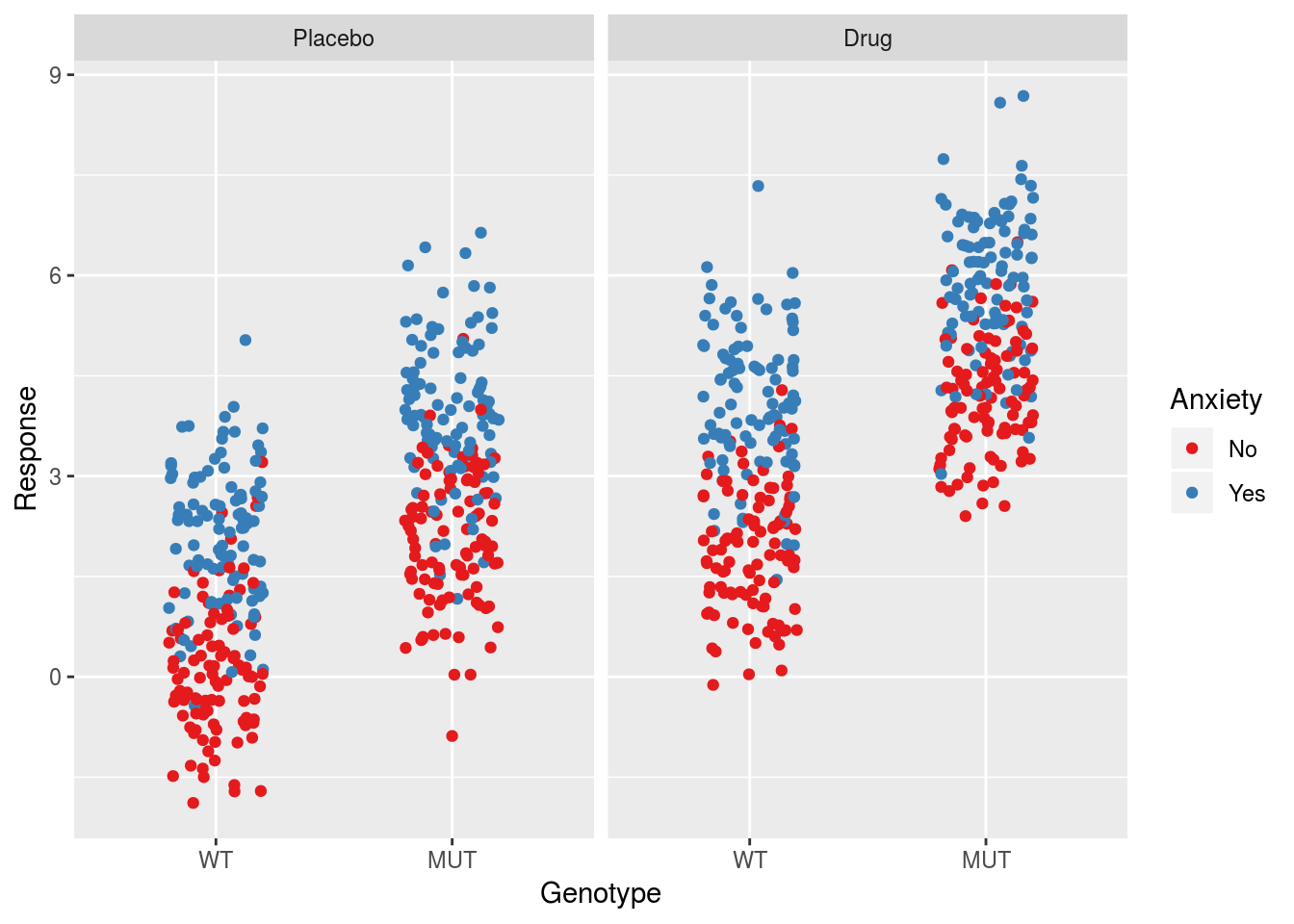
Here is the model:
linMod4 <- lm(Response ~ Genotype + Anxiety + Treatment, data = dfSimple)
summary(linMod4)
##
## Call:
## lm(formula = Response ~ Genotype + Anxiety + Treatment, data = dfSimple)
##
## Residuals:
## Min 1Q Median 3Q Max
## -2.9908 -0.6887 -0.0230 0.6759 3.3164
##
## Coefficients:
## Estimate Std. Error t value Pr(>|t|)
## (Intercept) 0.07123 0.07065 1.008 0.314
## GenotypeMUT 2.00231 0.07065 28.343 <2e-16 ***
## AnxietyYes 1.98574 0.07065 28.109 <2e-16 ***
## TreatmentDrug 1.96314 0.07065 27.789 <2e-16 ***
## ---
## Signif. codes: 0 '***' 0.001 '**' 0.01 '*' 0.05 '.' 0.1 ' ' 1
##
## Residual standard error: 0.9991 on 796 degrees of freedom
## Multiple R-squared: 0.7482, Adjusted R-squared: 0.7473
## F-statistic: 788.5 on 3 and 796 DF, p-value: < 2.2e-16Note that this is the proper model to describe the data based on how we’ve simulated it. In this case the intercept should describe the mean of the reference group, i.e. untreated wildtypes with no anxiety, while the slope parameters should estimate the inputs that we put into the model. The residuals standard error should describe the standard deviation of the response within the 8 different groups, which in this case amounts to the value of \(\sigma\) that we specified when simulating the data. The group standard deviations and their average are:
dfSimple %>%
  group_by(Genotype, Anxiety, Treatment) %>%
  summarise(varPerGroup = var(Response)) %>%
  ungroup %>%
  mutate(sigma = sqrt(mean(varPerGroup)))
## # A tibble: 8 x 5
## Genotype Anxiety Treatment varPerGroup sigma
## <fct> <fct> <fct> <dbl> <dbl>
## 1 WT No Placebo 1.01 0.996
## 2 WT No Drug 0.857 0.996
## 3 WT Yes Placebo 1.04 0.996
## 4 WT Yes Drug 1.11 0.996
## 5 MUT No Placebo 0.995 0.996
## 6 MUT No Drug 0.748 0.996
## 7 MUT Yes Placebo 1.14 0.996
## 8 MUT Yes Drug 1.04 0.996As expected the residual standard error is approximately the average of the group standard deviations.
What about the parameter errors?
xMat <- model.matrix(linMod4)
t(xMat) %*% xMat
## (Intercept) GenotypeMUT AnxietyYes TreatmentDrug
## (Intercept) 800 400 400 400
## GenotypeMUT 400 400 200 200
## AnxietyYes 400 200 400 200
## TreatmentDrug 400 200 200 400Which gives
\[\mathbf{X'X} = n \cdot \begin{bmatrix} 1 & \frac{1}{2} & \frac{1}{2} & \frac{1}{2} \\ \frac{1}{2} & \frac{1}{2} & \frac{1}{4} & \frac{1}{4} \\ \frac{1}{2} & \frac{1}{4} & \frac{1}{2} & \frac{1}{4} \\ \frac{1}{2} & \frac{1}{4} & \frac{1}{4} & \frac{1}{2} \end{bmatrix}\]
The full covariance matrix is then:
\[\sigma^2_\beta = \frac{\sigma^2}{n}\cdot\begin{bmatrix} 4 & -2 & -2 & -2 \\ -2 & 4 & 0 & 0 \\ -2 & 0 & 4 & 0 \\ -2 & 0 & 0 & 4 \end{bmatrix}\]
And the standard errors are:
\[\sigma_\beta = \frac{\sigma}{\sqrt{n}}\begin{bmatrix} \sqrt{4} & \sqrt{4} & \sqrt{4} & \sqrt{4} \end{bmatrix}\]
As we can see, the trend from the previous Section continues. The conversion factor for the intercept term is related to the number of parameters in the model, while the values related to the slope parameters are still simply \(\sqrt{4}\). We can expect that, as we continue to add binary predictors, the intercept term will be related to the number of parameters, while the slope parameters will have a conversion of \(\sqrt{4}\). As in the previous Sections, we can recover the residual standard error by multiplying by the appropriate factors:
vec <- c(sqrt(nObs/4), sqrt(nObs/4), sqrt(nObs/4), sqrt(nObs/4))
summary(linMod4)$coefficients[,"Std. Error"]*vec
## (Intercept) GenotypeMUT AnxietyYes TreatmentDrug
## 0.9990751 0.9990751 0.9990751 0.9990751Recap
At this stage let’s compare the conversion factors from \(\sigma\) to \(\sigma_\beta\) for all non-interactive models.
data.frame(Beta0 = c(1/sqrt(nObs), sqrt(2/nObs), sqrt(3/nObs), sqrt(nObs/4)),
           Beta1 = c(NA, sqrt(4/nObs), sqrt(4/nObs), sqrt(4/nObs)),
           Beta2 = c(NA, NA, sqrt(4/nObs), sqrt(4/nObs)),
           Beta3 = c(NA, NA, NA, sqrt(4/nObs)),
row.names = c("Model 1", "Model 2", "Model 3", "Model 4")) %>% kable()| Beta0 | Beta1 | Beta2 | Beta3 | |
|---|---|---|---|---|
| Model 1 | 0.0353553 | NA | NA | NA |
| Model 2 | 0.0500000 | 0.0707107 | NA | NA |
| Model 3 | 0.0612372 | 0.0707107 | 0.0707107 | NA |
| Model 4 | 14.1421356 | 0.0707107 | 0.0707107 | 0.0707107 |
As one might expect, we do see some pattern. Specifically, using the total number of observations, we can express this table as:
| Beta0 | Beta1 | Beta2 | Beta3 | |
|---|---|---|---|---|
| Model 1 | \(\sqrt{\frac{1}{n}}\) | NA | NA | NA |
| Model 2 | \(\sqrt{\frac{2}{n}}\) | \(\sqrt{\frac{4}{n}}\) | NA | NA |
| Model 3 | \(\sqrt{\frac{3}{n}}\) | \(\sqrt{\frac{4}{n}}\) | \(\sqrt{\frac{4}{n}}\) | NA |
| Model 4 | \(\sqrt{\frac{4}{n}}\) | \(\sqrt{\frac{4}{n}}\) | \(\sqrt{\frac{4}{n}}\) | \(\sqrt{\frac{4}{n}}\) |
As mentioned previously, the multiplicative factor for the intercept error involves the square root of the number of coefficients in the model. Moreover, for the rest of the models, the multiplicative factor is only ever \(\sqrt{\frac{4}{n}}\), i.e. the mappings don’t change as we add more binary variables. This makes sense given that all of the variables are independent in these models. Note that there is no pattern when expressing these conversion factors in terms of the number of data points per group, whic we will denote \(N\):
\[\begin{bmatrix} \sqrt{\frac{1}{N}} & & & \\ \sqrt{\frac{1}{N}}& \sqrt{\frac{2}{N}} & & \\ \sqrt{\frac{3}{4N}} & \sqrt{\frac{1}{N}} & \sqrt{\frac{1}{N}} & \\ \sqrt{\frac{1}{2N}} & \sqrt{\frac{1}{2N}} & \sqrt{\frac{1}{2N}} & \sqrt{\frac{1}{2N}} \end{bmatrix}\]
Recall that \(N\) here is different for each row, since the different models pool the data in different ways, and takes on values \(\{n, \frac{n}{2}, \frac{n}{4}, \frac{n}{8}\}\).
Interactive Models
In this Section we explore the influence of interactions on the parameter error estimates and the mapping from the residual standard error.
Two Binary Predictors with Interaction
In this case we consider the interaction between two of the variables, Genotype and Anxiety.
linModInt <- lm(Response ~ Genotype*Anxiety, data = dfSimple)
summary(linModInt)
##
## Call:
## lm(formula = Response ~ Genotype * Anxiety, data = dfSimple)
##
## Residuals:
## Min 1Q Median 3Q Max
## -4.0109 -1.0434 0.0248 1.0528 4.2269
##
## Coefficients:
## Estimate Std. Error t value Pr(>|t|)
## (Intercept) 0.98172 0.09903 9.913 <2e-16 ***
## GenotypeMUT 2.14447 0.14005 15.312 <2e-16 ***
## AnxietyYes 2.12790 0.14005 15.194 <2e-16 ***
## GenotypeMUT:AnxietyYes -0.28431 0.19806 -1.435 0.152
## ---
## Signif. codes: 0 '***' 0.001 '**' 0.01 '*' 0.05 '.' 0.1 ' ' 1
##
## Residual standard error: 1.4 on 796 degrees of freedom
## Multiple R-squared: 0.5053, Adjusted R-squared: 0.5034
## F-statistic: 271 on 3 and 796 DF, p-value: < 2.2e-16Note that though we have added a new predictor, there are still only 4 groups, as in Model 3. The difference is that the mean values of these groups may be more accurately estimated. In the present case we don’t expect this model to out-perform the model without an interaction, since there is no real interaction in the data, making the interaction parameter superfluous. This means that the estimate for the residual standard error should be similar to that from the non-interactive model. If the situation were reversed however and the data truly contained an interaction, then this model would more appropriately recapitulate the group means and lead to a more accurate estimation of \(\sigma\).
The design matrix will be different either way however due to the additional interaction predictor.
xMat <- model.matrix(linModInt)
t(xMat) %*% xMat
## (Intercept) GenotypeMUT AnxietyYes
## (Intercept) 800 400 400
## GenotypeMUT 400 400 200
## AnxietyYes 400 200 400
## GenotypeMUT:AnxietyYes 200 200 200
## GenotypeMUT:AnxietyYes
## (Intercept) 200
## GenotypeMUT 200
## AnxietyYes 200
## GenotypeMUT:AnxietyYes 200Explicitly using the observation number, we have:
\[n \cdot \begin{bmatrix} 1 & \frac{1}{2} & \frac{1}{2} & \frac{1}{4} \\ \frac{1}{2} & \frac{1}{2} & \frac{1}{4} & \frac{1}{4} \\ \frac{1}{2} & \frac{1}{4} & \frac{1}{2} & \frac{1}{4} \\ \frac{1}{4} & \frac{1}{4} & \frac{1}{4} & \frac{1}{4} \end{bmatrix}\]
The covariance matrix is:
\[\sigma^2_\beta = \frac{\sigma^2}{n}\cdot\begin{bmatrix} 4 & -4 & -4 & 4 \\ -4 & 8 & 4 & -8 \\ -4 & 4 & 8 & -8 \\ 4 & -8 & -8 & 16 \end{bmatrix}\]
with parameter standard errors of
\[\sigma_\beta = \frac{\sigma}{\sqrt{n}}\begin{bmatrix} \sqrt{4} & \sqrt{8} & \sqrt{8} & \sqrt{16} \end{bmatrix}\]
Here we see a pattern change from the models without an interaction. The intercept mapping still involves a scaling factor that uses the number of parameters in the model, but the standard errors for the main effects parameters are now larger by a factor of \(\sqrt{2}\) compared to the model without an interaction. The parameter error for the interaction is also larger than that for the main effects. These considerations will have a slight impact on the inferential side of linear modelling. Specifically, an interaction effect will always be less powerful than a main effect, and a main effect in a model with an interaction will always be less powerful than a main effect in a model without an interaction. The reason for this is that the \(t\)-statistic is computed as \(t = \hat{\beta}/\sigma_\beta\). Of course this depends on what model accurately describes the data. The aforementioned power of a non-interactive model will be thrown off on data with an interaction, since the estimate for \(\sigma\) will be larger due to the interaction in the data. These are things to keep in mind when considering which model to use.
Applying the mappings to the parameter standard errors, we recover the residual standard error:
vec <- c(sqrt(nObs/4), sqrt(nObs/8), sqrt(nObs/8), sqrt(nObs/16))
summary(linModInt)$coefficients[,"Std. Error"]*vec
## (Intercept) GenotypeMUT AnxietyYes
## 1.400499 1.400499 1.400499
## GenotypeMUT:AnxietyYes
## 1.400499Interaction without Main Effect
In this final Section I examine the interesting case of a model with a second order interaction but without the main effect for one of the predictors. What this model does is that it describes data in which the reference group for one of the binary variables (e.g. Wildtypes) is not influenced by observations of another variable (e.g. Anxiety). In order to get the lm() function to do this properly, we have to create an explicit dummy encoding of the variable with a main effect.
dfSimple <- dfSimple %>%
  mutate(GenotypeDummy = case_when(Genotype == "WT" ~ 0,
                                                          Genotype == "MUT" ~ 1))
linModInt2 <- lm(Response ~ GenotypeDummy + GenotypeDummy:Anxiety, data = dfSimple)
summary(linModInt2)
##
## Call:
## lm(formula = Response ~ GenotypeDummy + GenotypeDummy:Anxiety,
## data = dfSimple)
##
## Residuals:
## Min 1Q Median 3Q Max
## -4.0109 -1.1560 0.0171 1.1692 5.2909
##
## Coefficients:
## Estimate Std. Error t value Pr(>|t|)
## (Intercept) 2.04567 0.07948 25.737 < 2e-16 ***
## GenotypeDummy 1.08052 0.13767 7.849 1.35e-14 ***
## GenotypeDummy:AnxietyYes 1.84359 0.15897 11.597 < 2e-16 ***
## ---
## Signif. codes: 0 '***' 0.001 '**' 0.01 '*' 0.05 '.' 0.1 ' ' 1
##
## Residual standard error: 1.59 on 797 degrees of freedom
## Multiple R-squared: 0.3618, Adjusted R-squared: 0.3602
## F-statistic: 225.9 on 2 and 797 DF, p-value: < 2.2e-16Note that, in comparison to the fully interactive model presented in the previous Section, the residual standard error estimate is different. This is because the model has pooled the anxiety “yes” and “no” groups for the wildtypes. Since the data we generated included a main effect of anxiety, the variance of this wildtype group will be larger than that of the other two groups (mutant-no-anxiety and mutant-yes-anxiety). Additionally, the residual standard error is no longer just the average of the group standard deviations. This is due mainly to the fact that the wildtype group in this model is twice as large as the other two groups. To demonstrate this, let’s compute the naive average of group standard deviations:
(dfTemp <- dfSimple %>%
  mutate(NewGroups = case_when(Genotype == "WT" ~ "WT",
                               Genotype == "MUT" & Anxiety == "No" ~ "NoMUT",
                               Genotype == "MUT" & Anxiety == "Yes" ~ "YesMUT")) %>%
  group_by(NewGroups) %>%
  summarise(varPerGroup = var(Response)) %>%
  ungroup %>%
  mutate(sigma = sqrt(mean(varPerGroup))))
## # A tibble: 3 x 3
## NewGroups varPerGroup sigma
## <chr> <dbl> <dbl>
## 1 NoMUT 2.05 1.54
## 2 WT 3.01 1.54
## 3 YesMUT 2.04 1.54Observe that the wildtype standard deviation is larger than that for the other groups. The average is not equal to the residual standard error. It can be shown mathematically that in this case the residual standard error can be estimated approximately as
sqrt((1/4)*(dfTemp$varPerGroup[1] + dfTemp$varPerGroup[3] + 2*dfTemp$varPerGroup[2]))## [1] 1.589483An important point is that for the present data, this model is not homoscedastic, which is one of the assumptions underlying inferential statistics using linear models. To move forward we will generate a new data set in which there is no main anxiety effect, only an interaction. This makes it so that the group standard deviations will be approximately the same and put us back in the regime of homoscedasticity. Thus even though the wildtype group will have double the number of observations, the residual standard error will be approximately the average of the group standard deviations. We will ignore the presence of Treatment.
meanRef <- 0
sigma <- 1
effectGenotype <- 2
effectAnxiety <- 2

dfSimple <- dfSimple %>%
  mutate(Response = case_when(Genotype == "WT" ~ rnorm(nrow(.),meanRef,sigma),
                              Genotype == "MUT" & Anxiety == "No" ~ rnorm(nrow(.),meanRef + effectGenotype, sigma),
                              Genotype == "MUT" & Anxiety == "Yes" ~ rnorm(nrow(.), meanRef + effectGenotype + effectAnxiety, sigma)))


ggplot(dfSimple, aes(x = Genotype, y = Response, col = Anxiety)) +
  geom_jitter(width = 0.2) +
  scale_color_brewer(palette = "Set1")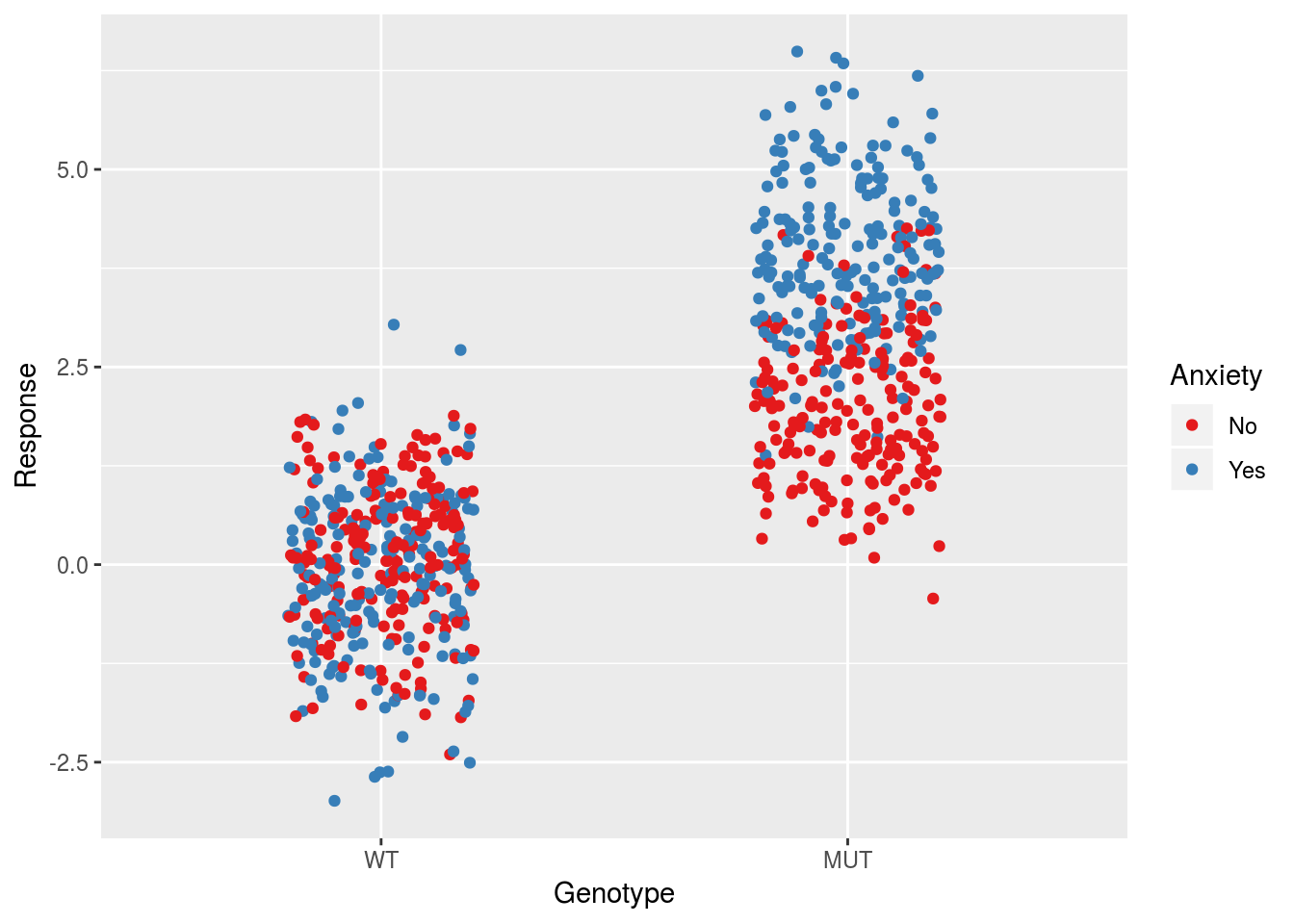
Re-running the model on this new data, we find:
dfSimple <- dfSimple %>% mutate(GenotypeDummy = case_when(Genotype == "WT" ~ 0,
                                                          Genotype == "MUT" ~ 1))
linModInt2 <- lm(Response ~ GenotypeDummy + GenotypeDummy:Anxiety, data = dfSimple)
summary(linModInt2)
##
## Call:
## lm(formula = Response ~ GenotypeDummy + GenotypeDummy:Anxiety,
## data = dfSimple)
##
## Residuals:
## Min 1Q Median 3Q Max
## -2.96592 -0.65534 0.00185 0.65837 3.05810
##
## Coefficients:
## Estimate Std. Error t value Pr(>|t|)
## (Intercept) -0.02255 0.04830 -0.467 0.641
## GenotypeDummy 2.00184 0.08366 23.927 <2e-16 ***
## GenotypeDummy:AnxietyYes 1.98251 0.09661 20.522 <2e-16 ***
## ---
## Signif. codes: 0 '***' 0.001 '**' 0.01 '*' 0.05 '.' 0.1 ' ' 1
##
## Residual standard error: 0.9661 on 797 degrees of freedom
## Multiple R-squared: 0.746, Adjusted R-squared: 0.7454
## F-statistic: 1170 on 2 and 797 DF, p-value: < 2.2e-16Note that the parameter estimates recapitulate what we put into the model. Moreover the residual standard error is now approximately equal to the input value of \(\sigma\). We can compute the group standard deviations to see how this relates to the residual standard error:
dfSimple %>%
  mutate(NewGroups = case_when(Genotype == "WT" ~ "WT",
                               Genotype == "MUT" & Anxiety == "No" ~ "NoMUT",
                               Genotype == "MUT" & Anxiety == "Yes" ~ "YesMUT")) %>%
  group_by(NewGroups) %>%
  summarise(varPerGroup = var(Response)) %>%
  ungroup %>%
  mutate(sigma = sqrt(mean(varPerGroup)))
## # A tibble: 3 x 3
## NewGroups varPerGroup sigma
## <chr> <dbl> <dbl>
## 1 NoMUT 0.846 0.963
## 2 WT 0.953 0.963
## 3 YesMUT 0.980 0.963In this case the average is closer to the residual standard error estimate.
Next we examine the mapping from \(\sigma\) to \(\sigma_\beta\) to see how it compares to the model with a main anxiety effect.
xMat <- model.matrix(linModInt2)
t(xMat) %*% xMat
## (Intercept) GenotypeDummy
## (Intercept) 800 400
## GenotypeDummy 400 400
## GenotypeDummy:AnxietyYes 200 200
## GenotypeDummy:AnxietyYes
## (Intercept) 200
## GenotypeDummy 200
## GenotypeDummy:AnxietyYes 200\[ n \cdot \begin{bmatrix} 1 & \frac{1}{2} & \frac{1}{4} \\ \frac{1}{2} & \frac{1}{2} & \frac{1}{4} \\ \frac{1}{4} & \frac{1}{4} & \frac{1}{4} \end{bmatrix}\]
The covariance matrix is
\[\frac{\sigma^2}{n}\cdot\begin{bmatrix} 2 & -2 & 0 \\ -2 & 6 & -4 \\ 0 & -4 & 8 \end{bmatrix}\]
which leads to standard errors of
\[\sigma_\beta = \frac{\sigma}{\sqrt{n}}\begin{bmatrix} \sqrt{2} & \sqrt{6} & \sqrt{8} \end{bmatrix}\]
Now, comparing this model to the previous model with both main effects:
data.frame(Intercept = c(sqrt(4/nObs),sqrt(2/nObs)),
           Genotype = c(sqrt(8/nObs), sqrt(6/nObs)),
           Anxiety = c(sqrt(8/nObs), NA),
           GenotypeAnxiety = c(sqrt(16/nObs), sqrt(8/nObs)),
           row.names = c("With Main Effect", "Without Main Effect"))
## Intercept Genotype Anxiety GenotypeAnxiety
## With Main Effect 0.07071068 0.10000000 0.1 0.1414214
## Without Main Effect 0.05000000 0.08660254 NA 0.1000000Using the number of observations \(n\) we find:
| Intercept | Genotype | Anxiety | GenotypeAnxiety | |
|---|---|---|---|---|
| With Main Effect | \(\sqrt{\frac{4}{n}}\) | \(\sqrt{\frac{8}{n}}\) | \(\sqrt{\frac{8}{n}}\) | \(\sqrt{\frac{16}{n}}\) |
| Without Main Effect | \(\sqrt{\frac{2}{n}}\) | \(\sqrt{\frac{6}{n}}\) | \(\sqrt{\frac{8}{n}}\) |
The patterns from the previous Sections break down in this case. Notably the conversion factor for the intercept term is no longer related to the number of parameters in the model. The standard errors for both the main effect and interaction term are also smaller in this model compared to the model with both main effects, assuming a fixed value of \(\sigma\). This does require caution however, as we saw that the residual standard error may be larger for this model if there is a actually a main effect in the data.
Conclusion
In conclusion, we recapitulate the \(\sigma\)-to-\(\sigma_\beta\) mappings for the different models that we considered:
| Intercept | Genotype | Anxiety | Treatment | GenotypeAnxiety | NumGroups | |
|---|---|---|---|---|---|---|
| Intercept Only | \(\sqrt{\frac{1}{n}}\) | NA | NA | NA | NA | 1 |
| One Binary Variable | \(\sqrt{\frac{2}{n}}\) | \(\sqrt{\frac{4}{n}}\) | NA | NA | NA | 2 |
| Two Binary Variables | \(\sqrt{\frac{3}{n}}\) | \(\sqrt{\frac{4}{n}}\) | \(\sqrt{\frac{4}{n}}\) | NA | NA | 4 |
| Three Binary Variables | \(\sqrt{\frac{4}{n}}\) | \(\sqrt{\frac{4}{n}}\) | \(\sqrt{\frac{4}{n}}\) | \(\sqrt{\frac{4}{n}}\) | NA | 8 |
| Interaction With Main Effect | \(\sqrt{\frac{4}{n}}\) | \(\sqrt{\frac{8}{n}}\) | \(\sqrt{\frac{8}{n}}\) | NA | \(\sqrt{\frac{16}{n}}\) | 4 |
| Interaction Without Main Effect | \(\sqrt{\frac{2}{n}}\) | \(\sqrt{\frac{6}{n}}\) | NA | NA | \(\sqrt{\frac{8}{n}}\) | 3 |
There are a few things to keep in mind. First, the standard deviation of the different groups is captured in the residual standard error estimate. Specifically if \(n \gg p\), this estimate is approximately equal to the average of the group sample standard deviations.
There is no obvious direct relationship between the standard errors of the parameters and the group standard deviations. For instance, the parameter error for the intercept is not equal to the standard error of the reference group, nor is the parameter error for the slope equal to the standard error of the non-reference group. The parameter errors depend on the non-trivial mapping \((\mathbf{X'X})^{-1}\).
There are however some patterns in the relationship for certain models. Specifically, for balanced binary variable models without interaction, the slope parameter standard errors are always related to the residual standard error by \(\sqrt{4/n}\), regardless of the number of binary variables in the model. The parameter error for the intercept does change however, and scales with the square root of the number of parameters in the model.
The patterns change when we add an interaction to the model. Comparing a two-variable model with an interaction to the corresponding model without an interaction, the parameters have larger errors in the interactive model. The interaction parameter is also the most uncertain parameter in the model. However the intercept parameter error still has a conversion factor related to the number of parameters in the model. If we remove one of the main effects from the model but maintain the interaction, all conversion factors shrink relative to the interactive model with the main effect. However this model should be used with caution as it will likely lead to grouping with uneven variances. On the other hand it can be a useful way to model data if one of the variables is not defined for one of the levels in the main effect, e.g. wildtypes without anxiety scores.
More complex interactive models were not explored in depth in this document, but for completion I will include the \(\sigma\)-to-\(\sigma_\beta\) mappings for two models. The two-variable interaction model described previously can be augmented to include a third variable. The complete interactive model at second order is as follows:
\[\text{Response} \sim \text{Genotype} + \text{Anxiety} + \text{Treatment} + \text{Genotype:Anxiety} + \text{Genotype:Treatment} + \text{Treatment:Anxiety}\]
The mapping for this model is:
\[\sigma_\beta = \frac{\sigma}{\sqrt{n}}\begin{bmatrix} \sqrt{7} & \sqrt{12} & \sqrt{12} & \sqrt{12}& \sqrt{16} & \sqrt{16} & \sqrt{16} \end{bmatrix}\]
The interactive model at the third order is:
\[\text{Response} \sim \text{Genotype} + \text{Anxiety} + \text{Treatment} + \text{Genotype:Anxiety} + \text{Genotype:Treatment} + \text{Treatment:Anxiety} + \text{Genotype:Anxiety:Treatment}\]
The mapping for this model is:
\[\sigma_\beta = \frac{\sigma}{\sqrt{n}}\begin{bmatrix} \sqrt{8} & \sqrt{16} & \sqrt{16} & \sqrt{16}& \sqrt{32} & \sqrt{32} & \sqrt{32} & \sqrt{64} \end{bmatrix}\]
The one thing I will mention about these mappings is that the conversion factors for the intercept standard errors continue to be related to the number of parameters in the model. There are likely other interesting patterns in these more complex interactive models, but these will not be explored here.
Ultimately these specific cases should serve to provide some intuition about how the parameter errors are estimated for a linear model. Keep in mind however that these mappings were computed for a balanced binary experimental design. Group imbalances will skew these values, though the size of these differences will depend on the degree of imbalance. Moreover the mappings will be different in the case of multi-level categorical variables and continuous numerical variables.